


This is an excerpt of the paper “Artificial intelligence for multimodal data integration in oncology”, published by “Cancer Cell” in OCTOBER 10, 2022.
Authored by: Jana Lipkova, Richard J. Chen, Bowen Chen, Ming Y. Lu, Matteo Barbieri, Daniel Shao, Anurag J. Vaidya, Chengkuan Chen, Luoting Zhuang, Drew F.K. Williamson, Muhammad Shaban, Tiffany Y. Chen, and Faisal Mahmood
Site Editor:
Joaquim Cardoso MSc
health transformation institute (HTI)
October 16, 2022
Key messages:
AI methods can be categorized as :
- supervised,
- weakly supervised, or
- unsupervised.
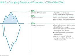
AI has the potential to have an impact on the whole landscape of oncology, ranging from prevention to intervention.
- AI models can explore complex and diverse data to identify factors related to high risks of developing cancer to support large population screenings and preventive care.
- The models can further reveal associations across modalities to help identify diagnostic or prognostic biomarkers from easily accessible data to improve patient risk stratification or selection for clinical trials.
- In a similar way, the models can identify non-invasive alternatives to existing biomarkers to minimize invasive procedures.
- Prognostic models can predict risk factors or adverse treatment outcomes prior to interventions to guide patient management.
- Information acquired from personal wearable devices or nanotechnologies could be further analyzed by AI models to search for early signs of treatment toxicity or resistance, with other great application yet to come.
AI methods in oncology [excerpt]
AI methods can be categorized as :
- supervised,
- weakly supervised, or
- unsupervised.
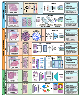
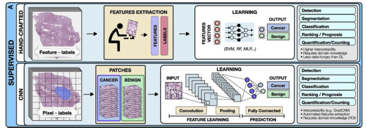
To highlight the concepts specific to each category we present all methods in the framework of computer vision as applied to digital pathology (Figure 2).
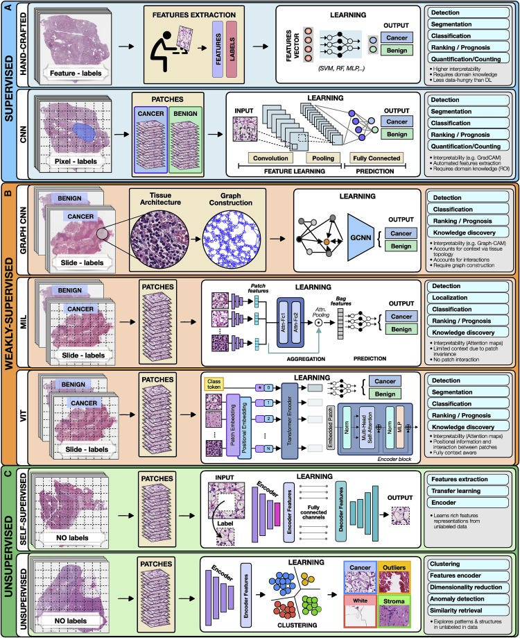
Figure 2. Overview of AI methods
(A) Supervised methods use strong supervision whereby each data point (e.g., feature or image patch) is assigned a label.
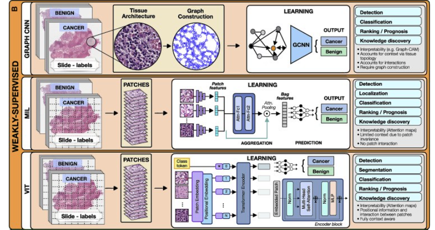
(B) Weakly supervised methods allow one to train the model with weak, patient-level labels, avoiding the need for manual annotations.
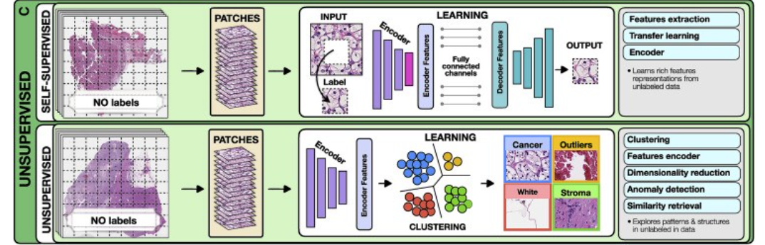
© Unsupervised methods explore patterns, subgroups, and structures in unlabeled data. For comparison, all methods are illustrated on a binary cancer detection task.
Supervised methods
Supervised methods map input data to predefined labels (e.g., cancer/non-cancer) using annotated data points such as digitized slides with pixel-level annotations, or radiology images with patient outcome.
Examples of fully supervised methods include hand-crafted and representation learning methods.
- Hand-crafted methods
- Representation learning methods
a.Hand-crafted methods
These methods take as input a set of predefined features (e.g., cell shape or size) extracted from the data before the training, not the data themselves.
The training is performed with standard machine-learning (ML) models, such as random forest (RF), support-vector machine (SVM), or multilayer perceptron (MLP) (Bertsimas and Wiberg, 2020) (Figure 2).
Since the feature extraction is not part of the learning process, the models typically have simpler architecture, lower computation cost, and may require less training data than DL models.
An additional benefit is a high level of interpretability, since the predictive features can be related to the data.
On the other hand, the feature extraction is time consuming and can translate human bias to the models.
A downside is that manual feature extraction or engineering limits the models ability to features already known and understood by humans and prevents the utility and downstream discovery of new relevant features.
Moreover, human perception cannot be easily captured by a set of mathematical operators, often leading to simpler features.
Since the features are usually tailored to the specific disease, the models cannot be easily translated to other tasks or malignancies.
Despite the popularity of DL methods, in many applications the hand-crafted methods are sufficient and preferred due to their simplicity and ability to learn from smaller datasets.
b.Representation learning methods
Representation learning methods such as deep learning (DL) are capable of learning rich feature representations from the raw data without the need for manual feature engineering.
Here we focus on convolutional neural networks (CNNs), the most common DL strategy for image analysis. In CNNs the predictive features are not defined, and the model learnins which concepts and features are useful for explaining relations between inputs and outputs.
For instance, in Figure 2, each training whole-slide image (WSI) is manually annotated to outline the tumor region. The WSI is then partitioned into rectangular patches and each patch is assigned with a label, “cancer” or “no-cancer,” determined by the tumor annotation.
The majority of CNNs have similar architectures, consisting of alternating convolutional, pooling, and non-linear activation layers, followed by a small number of fully connected layers.
A convolution layer serves as a feature extractor, while the subsequent pooling layer condenses the features into the most relevant ones.
The non-linear activation function allows the model to explore complex relations across features. Fully connected layers then perform the end task, such as classification.
The main strength of CNNs is their ability to extract rich feature representations from raw data, resulting in lower preprocessing cost, higher flexibility, and often superior performance over hand-crafted models.
The potential limitations come from the model’s reliance on pixel-level annotations, which are time intensive and might be affected by interrater variability and human bias.
Moreover, predictive regions for many clinical outcomes, such as survival or treatment resistance, may be unknown.
CNNs are also often criticized for their lack of interpretability, while we are able to often examine regions used by the model to make predictive determinations, the overall feature representations remain abstract.
Despite these limitations, CNNs come with impressive performance, contributing to widespread usage in many clinically relevant applications.
2.Weakly supervised methods
Weakly supervised learning is a sub-category of supervised learning with batch annotations on large clusters of data essentially representing a scenario where the supervisory signal is weak compared to the amount of noise in the dataset.
A common example of the utility of weak supervision is detection of small tumor regions in a biopsy or resection in a large gigapixel whole slide image with labels at the level of the slide or case.
Weakly supervised methods allow one to train models with weak, patient-level labels (such as diagnosis or survival), avoiding the need for manual data annotations.
The most common weakly supervised methods include graph convolutional networks (GCNs), multiple-instance learning (MIL), and vision transformers (VITs).
- Graph convolutional networks
- Multiple-instance learning
- Vision transformers
a.Graph convolutional networks
Graphs can be used to explicitly capture structure within data and encode relations between objects making them ideal for analysis of tissue biospy images.
A graph is defined by nodes connected by edges.
In histology, a node can represent a cell, an image patch, or even a tissue region.
Edges encode spatial relations and interactions between nodes (Zhang et al., 2019).
The graph, combined with the patient-level labels, is processed by a GCN (Ahmedt-Aristizabal et al., 2021), which can be seen as a generalization of CNNs that operate on unstructured graphs.
In GCNs, feature representations of a node are updated by aggregating information from neighboring nodes. The updated representations then serve as input for the final classifier (Figure 2).
GCNs can incorporate larger context and spatial tissue structure as compared to a conventional deep models for digital pathology which patch the image into small regions which remain mutually exclusive.
This can be beneficial in tasks where the spatial context spans beyond the scope of a single patch (e.g., Gleason score).
On the other hand, the interdependence of the nodes in GCNs comes with higher training costs and memory requirements, since the nodes cannot be processed independently.
b.Multiple-instance learning
MIL is a type of weakly supervised learning where multiple instances of the input are not individually labeled and the supervisory signal is only available collectively for a set of instances commonly reffered to as a bag (Carbonneau et al., 2018; Cheplygina et al., 2019)
The label of a bag is assumed positive if there is at least one positive instance in the bag.
The goal of the model is to predict the bag label. MIL models comprise three main modules: feature learning or extraction, aggregation, and prediction.
The first module is used to embed the images or other higher dimentional data into lower-dimensional embeddings this module can be trained on the fly (Campanella et al., 2019) or a pre-trained encoder from supervised or self-supervised learning can be used to reduce training time and data-efficiency (Lu et al., 2021).
The instance-level embeddings are aggregated to create patient-level representations, which serve as input for the final classification module.
A commonly used aggrigation stratergy is attention-based pooling, (Ilse et al., 2018), where two fully connected networks are used to learn the relative importance of each instance (Ilse et al., 2018).
The patch-level representations, weighted by the corresponding attention score, are summed up to build the patient-level representation.
The attention scores can be also be used in understanding the predictive basis of the model (see “multimodal interpretability” for additional details).
In large scale medical datasets fine annotations are often not available which makes MIL an ideal approach for training deep models, there are several recent examples in cancer pathology (Campanella et al., 2019, Lu et al., 2021, Lu et al., 2021) and genomics (Sidhom et al., 2021).
c.Vision transformers
VITs (Dosovitskiy et al., 2020; Vaswani et al., 2017) are a type of attention-based learning which allows for the model to be fully context aware.
In contrast to MIL, where patches are assumed independent and identically distributed, VITs account for correlation and context among patches.
The main components of VITs include positional encoding, self-attention, and multihead self-attention.
Positional encoding learns the spatial structure of the image and the relative distances between patches.
The self-attention mechanism determines the relevance of each patch while also accounting for the context and contributions from the other patches.
Multihead self-attention simultaneously deploys multiple self-attention blocks to account for different types of interactions between the patches and combines them into a single self-attention output.
A typical VIT architecture is shown in Figure 2. A WSI is converted into a series of patches, each coupled with positional information.
Learnable encoders map each patch and its position into a single embedding vector, referred to as a token.
An additional tokens is introduced for the classification task.
The class token together with the patch tokens is fed into the transformer encoder to compute multihead self-attention and output the learnable embeddings of patches and the class.
The output class token serves as a slide-level representation used for the final classification.
The transformer encoder consists of several stacked identical blocks.
Each block includes multihead self-attention and MLP, along with layer normalization and residual connections.
The positional encoding and multiple self-attention heads allow one to incorporate spatial information, increase the context and robustness (Li et al., 2022; Shamshad et al., 2022) of VIT methods over other methods.
On the other hand, VITs tend to be more data hungry (Dosovitskiy et al., 2020), a limitation that the machine learning community is actively working to overcome.
Weakly supervised methods offer several benefits.
The liberation from manual annotations reduces the cost of data preprocessing and mitigates the bias and interrater variability.
Consequently, the models can be easily applied to large datasets, diverse tasks, and also situations where the predictive regions are unknown.
Since the models are free to learn from the entire scan, they can identify predictive features even beyond the regions typically evaluated by pathologists.
The great performance demonstrated by weakly supervised methods suggests that many tasks can be addressed without expensive manual annotations or hand-crafted features.
3.Unsupervised methods
Unsupervised methods explore structures, patterns, and subgroups in data without relying on any labels. These include self-supervised and fully unsupervised strategies.
- Self-supervised methods
- Unsupervised feature analysis
a.Self-supervised methods
Self-supervised methods aim to learn rich feature representations from within data by posing the learning problem as a task the ground truth for which is defined within the data.
Such encoders are often used to obtain high quality lower dimentional embeddings of complex high dimentional datasets for making downstream tasks more efficient interms of data and training efficiency.
For example in pathology images self-supervised methods exploit available unlabeled data to learn high-quality image features and then transfer this knowledge to supervised models.
To achieve this, supervised methods such as CNNs are used to solve various pretext tasks (Jing and Tian, 2019) for which the labels are generated automatically from the data.
For instance, a patch can be removed from an image and a deep network is trained to predict the missing part of the image from its surroundings, using the actual patch as a label (Figure 2).
The patch prediction has no direct clinical relevance, but it guides the model to learn general-purpose features of image characteristics, which can be beneficial for other practical tasks.
The early layers of the network are usually capture general image features, while the later layers pick features relevant for the task at hand.
The later layers can be excluded, while the early layers serve as feature extractors in for supervised models (i.e., transfer learning).
b.Unsupervised feature analysis
These methods allow for exploring structure, similarity and common features across data points.
For example, using embeddings from a pre-trained encoder one could extract features from a large dataset of diverse patients and cluster said embeddings to find common features across the entire patient cohorts.
The most common unsupervised methods include clustering and dimensionality reduction. Clustering methods (Rokach and Maimon, 2005) partition data into subgroups such that the similarities within the subgroup and the separation between subgroups are maximized.
Although the output clusters are not task specific, they can reveal different cancer subtypes or patient subgroups.
The aim of dimensionality reduction is to obtain low-dimensional representation capturing the main characteristics and correlations in the data.
References and additional information:
See the original publication
Originally published at https://www.cell.com.
About the authors & affiliations:
Jana Lipkova,1,2,3,4
Richard J. Chen,1,2,3,4,5
Bowen Chen,1,2,8
Ming Y. Lu,1,2,3,4,7
Matteo Barbieri,1
Daniel Shao,1,2,6
Anurag J. Vaidya,1,2,6
Chengkuan Chen,1,2,3,4
Luoting Zhuang,1,3
Drew F.K. Williamson,1,2,3,4
Muhammad Shaban,1,2,3,4
Tiffany Y. Chen,1,2,3,4 and
Faisal Mahmood1,2,3,4,9, *
1 Department of Pathology,
Brigham and Women’s Hospital, Harvard Medical School, Boston, MA, USA
2Department of Pathology,
Massachusetts General Hospital, Harvard Medical School, Boston, MA, USA
3Cancer Program,
Broad Institute of Harvard and MIT, Cambridge, MA, USA
4Data Science Program,
Dana-Farber Cancer Institute, Boston, MA, USA
5Department of Biomedical Informatics,
Harvard Medical School, Boston, MA, USA
6 Harvard-MIT Health Sciences and Technology (HST), Cambridge, MA, USA
7Department of Electrical Engineering and Computer Science, Massachusetts Institute of Technology (MIT), Cambridge, MA, USA
8Department of Computer Science,
Harvard University, Cambridge, MA, USA
9 Harvard Data Science Initiative,
Harvard University, Cambridge, MA, USA