


a checklist for Ruling Out Bias Using Standard Tools in Machine Learning (ROBUST-ML)
European Heart Journal — Digital Health
Volume 3, Issue 2, June 2022
Salah S Al-Zaiti, Alaa A Alghwiri, Xiao Hu, Gilles Clermont, Aaron Peace, Peter Macfarlane, Raymond Bond
Executive Summary by
Joaquim Cardoso MSc.
Health Transformation — Strategy Advisory Consulting
AI Augmented Health Care Institute
July 13, 2022
Abstract
Developing functional machine learning (ML)-based models to address unmet clinical needs requires unique considerations for optimal clinical utility.
Recent debates about the rigours, transparency, explainability, and reproducibility of ML models, terms which are defined in this article, have raised concerns about their clinical utility and suitability for integration in current evidence-based practice paradigms.
This featured article focuses on increasing the literacy of ML among clinicians by providing them with the knowledge and tools needed to understand and critically appraise clinical studies focused on ML.
A checklist is provided for evaluating the rigour and reproducibility of the four ML building blocks: data curation, feature engineering, model development, and clinical deployment.
Checklists like this are important for quality assurance and to ensure that ML studies are rigourously and confidently reviewed by clinicians and are guided by domain knowledge of the setting in which the findings will be applied.
Bridging the gap between clinicians, healthcare scientists, and ML engineers can address many shortcomings and pitfalls of ML-based solutions and their potential deployment at the bedside.
Selected images
Figure 2 -The complexity of decisions considered when designing a machine learning model.
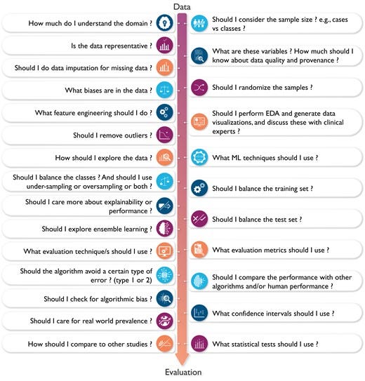
Figure 3 — Relationship between artificial intelligence, machine learning, and deep learning.
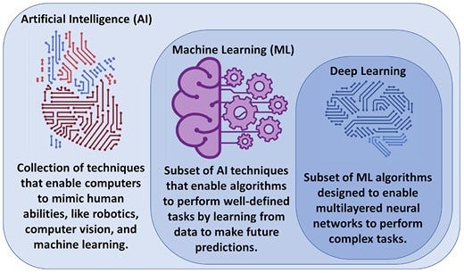
Figure 6 — summarizes the four main building blocks of a ML pipeline.
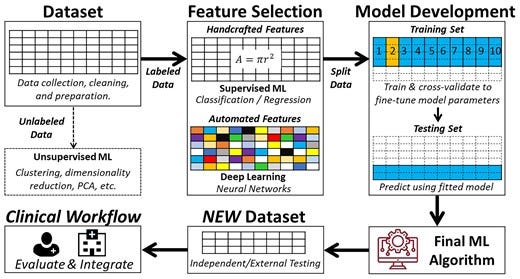
Figure 7
7a — Such ‘noise’ causes the model to overfit the training data, so it generalizes poorly to new data
7b — There is a tradeoff between bias and variance
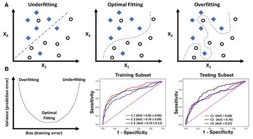
Figure 8 — shows a hypothetical tradeoff between model accuracy and mode explainability.
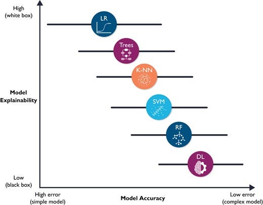
Table 7 — A checklist for Ruling Out Bias Using Standard Tools in Machine Learning
ORIGINAL PUBLICATION (full version)

Introduction
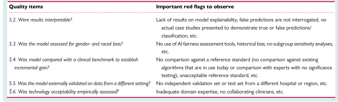
Machine learning (ML) is a field that lies at the intersection of mathematics and computer science, integrating principles from computing, optimization, and statistics. Successive advances in this field over the past few decades have brought a suite of very powerful mathematical algorithms able to learn hidden patterns from large quantities of data. From a data science-oriented perspective, ML is simply a collection of mathematical theories and statistical techniques that enable machines to improve at undertaking a given task with experience (e.g. recognition, prediction, prescription). Given that recognition and prediction are the backbone of clinical practice, many of these ML algorithms have proven efficient in addressing some longstanding challenges frequently encountered in analysing high dimensional, complex clinical data.1–6 These promising potentials have led to a rapid expansion in the number of articles published in clinical journals that focus on ML. Figure 1 shows the number of clinical diagnostic accuracy studies published in PubMed between 2000 and 2021 and the sub-portion of these studies that use ML methods. These trends translate to an annual growth rate of 8% compared with 39%, respectively. It is reported that nearly 25% of all diagnostic accuracy studies submitted to leading journals focus on the performance of ML algorithms.7 This is one in four papers in any given field to which an average clinician could be exposed.
Figure 1
Temporal trends in machine learning-centered articles published in PubMed between 2000 and 2021. This figure shows the results of a simple search on PubMed for clinical diagnostic studies focused on ‘diagnosis’ between 2000 and 2021 (line with square markers) and the sub-portion of those studies that reference ‘machine learning’, ‘artificial intelligence’, or ‘deep learning’ in the title or abstract (line with diamond markers).
This exponential growth in the use of ML techniques to address unmet clinical needs has not been effectively translated to the bedside due to many scientific, technical, and logistical challenges, dampening the enthusiasm by many healthcare providers. First, as target end-users at the bedside, many clinicians are not familiar with the concepts of ML and whether its applications in healthcare can be trusted. This could create a barrier to change and limit the potential deployment at the bedside. Many reviewers or editors of medical journals are also not very familiar with such ML methodologies. In an interesting experiment at a ML-focused conference (NeurIPS), double-blinded reviewers failed to reach consensus on more than 57% of submitted papers at 22.5% acceptance rate.8 Such a large margin of disagreement among reviewers might deter journals from accepting high-quality ML papers, or more worrisome, publish poorly performed or flawed ones. Second, because of this gap in common language between end-users and developers, clinicians are rarely integral members of data science teams, potentially diminishing the clinical relevance, model explainability, and workflow compatibility of many ML-centered solutions.9 Finally, the field of ML itself continues to suffer from shortcomings that have led to hot debates about its usefulness in recent years, including the black box label as well as gender and racial bias to mention a few.10,11 These concerns, coupled with the lack of a clear regulatory pathway12 and poor access to large and high-quality datasets, have limited the availability of approved ML-based medical devices in the USA and Europe, creating a clinical paradigm with sceptical stakeholders and growing mistrust between clinicians and ML applications.
Understanding the complexity (and subjectiveness) of modelling decisions involved in building a functional ML application is central to critically appraising clinical ML studies. Figure 2 showcases the kind of ‘decisions’ that each data scientist typically considers throughout the various steps of designing a ML pipeline (i.e. from data to decisions). This featured article focuses on increasing literacy of ML among clinicians by providing them with the knowledge and tools needed to understand and critically appraise clinical studies focused on ML. Clinical applications of ML in cardiovascular disease and cardiac imaging have been described in detail elsewhere.3 Herein, we provide a succinct review of commonly used ML techniques and best practices and considerations for building and translating effective ML models. We also highlight the most crucial design flaws and serious red flags for clinicians to consider while critically appraising ML-centered articles in healthcare.
Figure 2
The complexity of decisions considered when designing a machine learning model. This figure showcases the complexity and subjectiveness in the questions/decisions the data scientist may consider when building a machine learning algorithm. Ideally, these important decisions need to be made in conjunction with collaborating clinicians to enhance clinical relevance and utility. EDA, exploratory data analysis.
Basic definitions and terminologies
Artificial intelligence (AI) is the machine’s ability to mimic humans in learning and behaviour with automatic improvement and without explicit programming. Artificial intelligence encompasses multiple fields, including computer vision, robotics, and ML.13 Machine learning as a subfield of AI entails a collection of computer algorithms developed to automate regular processes and services or predict and forecast events of interest in a certain domain quickly and accurately using previously recorded historical data of that event. In healthcare, ML has been extensively used for clinical diagnostics, early prediction of outcomes, and disease phenotyping.14 Deep learning (DL), on the other hand, is a subclass of ML algorithms (i.e. multi-layered neural networks) that are designed to learn complex tasks from massive amounts of structured and unstructured data types like video, voice, image, or text.13Figure 3 visualizes the relationship between AI, ML, and DL as interrelated and overlapping fields.
Figure 3
Relationship between artificial intelligence, machine learning, and deep learning. Artificial intelligence is the general umbrella that encompasses machine learning with other domains, whereas deep learning is a subclass of machine learning algorithms (Credit: Salah Al-Zaiti. Created with BioRender.com).
Artificial intelligence was born back in the 1950s when a group of computer scientists started exploring whether computers could be designed to ‘think’ like humans. Early chess programmes are a good example of scientists’ first attempts of making computers act like humans. In this case, the programme involved hardcoded rules without any interactive learning. This approach, at that time, was called symbolic AI and dominated the field from the 1950s to the 1980s. Although symbolic AI proved to be a good approach to solve well-defined and logical problems, it turned out to be ill-suited to solving more complex and fuzzy problems such as image classification, speech recognition, and language translation. In late 1980s, ML arose to replace symbolic AI in automating intellectual tasks normally performed by human intelligence.
The concept behind ML algorithms is distinct from the rule-based logic seen in symbolic AI. Rather than programming a set of conditional statements derived from domain knowledge to guide decision making, scientists feed data rather than rules to train the model, refine its parameters, and test its performance for a given task (i.e. interactive learning). This model is then built in production. A key difference here is that rule-based algorithms use current knowledge already adopted by clinicians when making a decision (e.g. diagnosis), whereas a ML approach might use different rules or ‘features’ that it discovered during the data-driven process of model development. If we consider the task of diagnosing acute myocardial infarction (MI) using electrocardiogram (ECG) data as an example, a rule-based automated interpretation system would follow programmed rules like if ST amplitude ≥ 0.1 mV, then print ‘>>>Acute MI<<<’. On the contrary, a ML-based model would ‘learn’ the features and data-driven decision rules for classifying ‘>>>Acute MI<<<’ from an existing and labelled ECG dataset without any preexisting domain knowledge. The performance of this model is then tested on new ECG tracings not included in the original datasets. This is analogous to a cardiology fellow who is learning to read ECGs by reviewing few thousand examples under supervision until mastering his/her own unique approach; before interpreting ECGs in a real-world setting on his own.
The question then remains how ML is different from statistics used in the general medical literature. The main task of both is to find a mathematical representation in a multidimensional probability distribution, yet the focus and degree of formal development between both are different. Statistics is a branch of applied probabilities with well-outlined theoretical concepts focusing on drawing population inferences from sample data to understand the causal relationship between the predictors and the outcome variable (i.e. knowledge discovery to increase our understanding of a given phenomenon).15 For example, a statistician might explore the relationship between the presence of comorbidities and incidental cardiovascular disease using logistic regression. Here, the interest is inferring a function that can explain the most variability in incidental cardiovascular disease using a parsimonious subset of comorbidities, which would contribute to our understanding of disease pathogenesis (i.e. reduced dimensionality for knowledge discovery).16 On the other hand, ML uses general-purpose mathematical learning algorithms (beyond probabilities) to find generalizable patterns in high-dimensional data space without requiring prior assumptions about either the population or the residuals. In the previous example, a data scientist would explore a suite of learning models (which might include logistic regression) to build a model that yields the highest classification performance (i.e. sensitivity and specificity), with little attention to the impact of data properties on population density functions (i.e. no inferences). Here the interest is to find the model that best learns generalizable rules when applied to new unseen data (i.e. prediction rather than comprehension).15,17 Nevertheless, statistics and ML share numerous principles and techniques, and the overlap between both sometimes might be difficult to delineate. In fact, it has been shown that adapting statistical inferential techniques in learning algorithms (i.e. causal ML) dramatically boosts ML model performance.18
Subtypes of machine learning models
Machine learning models can be classified into four subtypes based on the degree of human supervision applied on data: supervised, unsupervised, semi-supervised, and reinforcement learning (RL).
In supervised learning, a set of input variables is used to predict an outcome of interest that has been labelled by experts.
Supervised techniques can be broken down into two subtypes according to the level of measurement of the outcome variable: regression or classification. In regression, the outcome is measured as a continuous numeric variable such as blood pressure, BMI, height, or weight. A regular prediction algorithm, such as linear regression or regression trees, is used when input data are collected at one time. If input data are longitudinal (i.e. time-series), then forecasting algorithms such Auto-Regressive Integrated Moving Average or exponential smoothing models could be used. In classification, the outcome of interest is measured as a categorical variable at either two levels (binary) or more (ordinal or nominal).
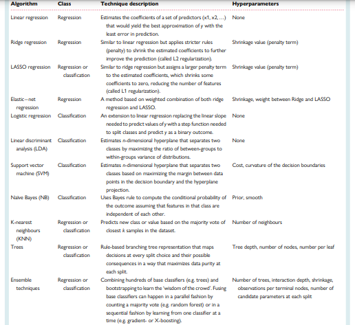
Table 1 summarizes the commonly used regression and classification techniques in supervised ML. This table also summarizes the adjustable free parameters needed to optimize each model performance (i.e. hyperparameters). Hyperparameters refer to the configurations of a model’s architecture that cannot be inferred from the data and need to be arbitrarily decided by the data scientist.
For instance, when building a simple decision tree, the data scientist needs to decide on the tree depth (number of levels) and number of nodes (decision splits) before a tree can be built. The selection of these hyperparameters is arbitrary and can be done by searching all potential combinations of hyperparameters that perform best on the historical data. Finding the best hyperparameters plays an important role in optimizing the goodness-of-fit on the sample data, ideally leading to good performance when generalized to new unseen data.
Table 1 — Common supervised machine learning techniques used in healthcare
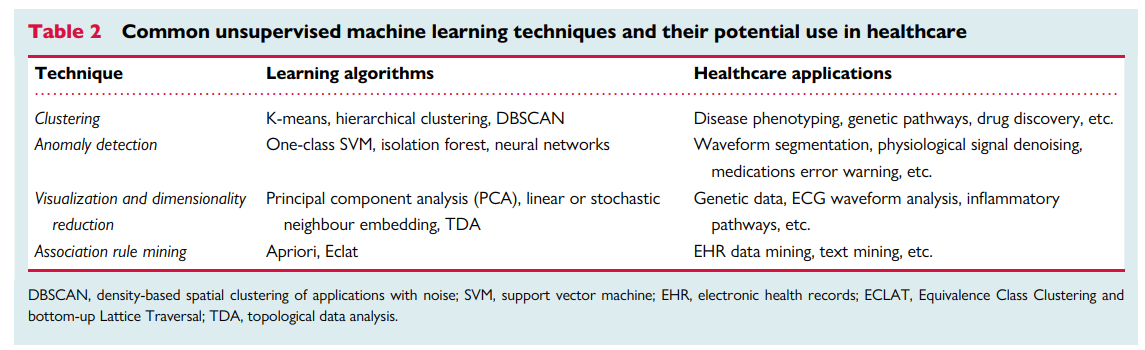
The second subtype of ML models is unsupervised learning where an algorithm autonomously draws associations from unlabelled data without any a priori knowledge of true labels. With the emergence of big data, data sources became massive, making labelling labour-intensive, time-consuming, and very costly. With the wide availability of such massive quantities of unlabelled training data, unsupervised learning techniques become essential. Table 2 summarizes the four most common unsupervised techniques along with their potential applications in healthcare. Clustering entails grouping together patients with approximately similar characteristics given a set of features. The emerging clusters can potentially identify unique phenotypes of a given disease. A clustering example would be grouping patients with chest pain based on their age, sex, risk factors, symptoms, lab tests, medications, and angiographic findings. The resulting clusters can then be used to identify specific phenotypes like Type 1 vs. Type 2 MI. Anomaly detection entails learning the baseline pattern of how features typically aggregate in order to identify potential deviations from this normal state. An example of anomaly detection would be learning certain clinical contexts when medication X is prescribed to a given patient so any new deviations from this norm can be flagged as a potential medication error. Dimensionality reduction entails the mathematical summarization of data across features using orthogonal (independent) vectors for simplified modelling and visualization. For instance, principal component analysis has been historically used to summarize ECG waveform data from 192 body surface potential maps (BSPM) to yield only 12 independent waveforms that capture >90% of prognostic information in the data, significantly enhancing the clinical utility of BSPM for bedside care. Finally, association rule mining entails approaches to learn strong rules with interesting relationships between-groups of variables in large datasets. For example, implementing an apriori algorithm on electronic health record data in an emergency department might yield the rule (chest pain, ECG) → (troponin), indicating that a chief complaint of chest pain with documented ECG record are pre-requisites to the availability of troponin results in the medical charts.
Table 2
Common unsupervised machine learning techniques and their potential use in healthcare
A third subtype of ML models is semi-supervised learning.
Despite the scarcity of labelled data in many fields (e.g. medical images, ECG signals), many datasets contain a mixture of both labelled and unlabelled data, which created an opportunity for leveraging techniques from both supervised and unsupervised learning. These new semi-supervised learning techniques are broadly grouped under two general umbrellas: self-learning algorithms and co-learning algorithms.19 In self-learning, a single classifier is trained on a small subset of ‘seed’ data then used to classify unlabelled data. Data points classified with high confidence are added to the ‘seed’ subset and the base classifier is re-trained. This iterative process continues until all data points are labelled. This technique has been successfully implemented in image classification.20 In co-learning, a similar approach is used to train three classifiers, rather than one, on the ‘seed’ subset, and then using the consensus of the three algorithms in order to add new data points to the ‘seed’ set before re-training. This technique has been successfully used for classifying the level of activity of a patient using motion data from cameras and sensors to monitor and determine when assistance is needed (e.g. after falling).21 Unlike self-learning and co-learning, a more novel approach is to train a single classifier on a ‘seed’ set, then use this model to select the data points with the lowest confidence in prediction and thereafter ask users to manually label these informative examples before adding them to the ‘seed’ set and re-training the classifier. This latter approach is called active learning and has been successfully used in ECG beat classification, image classification, gene expression, and artefact detection.22,23
A fourth subtype of learning models is RL, which constitutes a totally different paradigm in terms of how the model learns.
In general, there will be an agent which observes and learns the best policy (e.g. decision rules) by weighing actions (e.g. available treatment options) against subsequent rewards (e.g. short-term patient outcomes) where the policy can be adapted over time. Reinforcement learning is widely used in robotics, gaming, computer vision, and autonomous control.24 In healthcare, applications of RL are limited because its techniques warrant due diligence. Some of the successful applications include HIV therapy optimization, seizure control, and sepsis management.25 Reinforcement learning is a complex topic and has been explained in detail elsewhere.26
Finally, although not a distinct subtype of learning approaches, it is worth noting that DL has wide applications across supervised regression and classification, unsupervised, and semi-supervised learning, as well as RL.
As illustrated in Figure 4, the architecture of DL is based on a neural network composed of an input layer (features), hidden layers (function nodes), and an output layer (prediction). Input features can either be structured data elements or unstructured data (e.g. pixels). The functional unit at each ‘synaptic connection’ is called a neuron and includes a summation and activation functions. A ML engineer will first need to define the network architecture and hyperparameters (e.g. number of hidden layers, number of nodes per layer, type of activation function, connection topologies, etc.). The next and most computationally exhaustive task is optimizing the synaptic weights in each neuron, which is frequently achieved using an optimization approach called gradient descent. Calculating the weights that optimize gradient descent is done using a first order iterative technique called backpropagation. Deep learning is a complex topic and has been explained in detail elsewhere,27 but Table 3 provides a simple summary of the common DL algorithms generally used in medical literature.
Figure 4
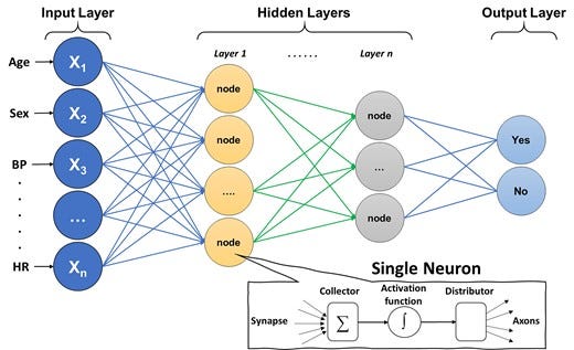
Basic architecture of a deep neural network. The figure shows the basic architecture of a deep neural network, which is composed of an input layer (features), hidden layers (function nodes), and an output layer (prediction). The functional unit at each ‘synaptic connection’ is called a neuron and includes a summation and activation functions.
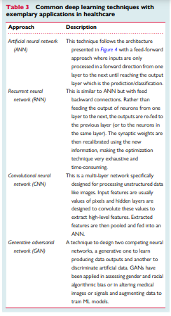
Table 3
Common deep learning techniques with exemplary applications in healthcare
A DL technique that is widely used in cardiovascular literature is convolutional neural networks (CNN). This technique is specifically useful for image and signal processing where a series of convolution and pooling layers are used to extract numeric features from the unstructured images and use these extracted features in a multi-layer ANN. Figure 5 shows a simple illustration of a CNN model with one convolution layer and one pooling layer. Briefly, an image is usually stored as n-dimensional byte array with a colour value of each pixel for each of the three main colour channels: red, green, and blue (i.e. RGB image). First, a Kaufman filter (i.e. Kernel) of a given matrix size (e.g. 3 × 3) hovers over each colour channel and the resulting multiplication of pixel values and kernel values is stored in a new byte array. This step is called ‘convolution’ and is used to extract the low-level features of the image (e.g. edges, gradient). Next, to reduce the spatial dimensionality of the byte arrays, adjacent pixel values in a given size (e.g. 2 × 2) are summarized together by using either the mean or the max value (i.e. average pooling or max pooling, respectively). This step is called ‘pooling’ and is useful for extracting dominant features. After a series of iterations between convolution and pooling layers, the resulting byte array can be flattened into n × 1 array and fed into a classical multi-layer ANN to train the model on classifying the images based on known outcomes of interest.
Figure 5
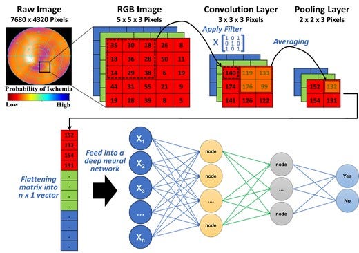
Basic architecture of a convolutional neural network. This figure illustrates how features can be extracted from a raw image (e.g. single photon emission computed tomography myocardial perfusion scan) for use in a neural network. The pixel values in each colour channel are multiplied by a kernel filter to extract low-level image features (convolution layer). Next, adjacent pixel values are grouped together using mean or max value to reduce spatial dimensionality (pooling layer). After repeated iterations of these two layers, the final byte array matrix is flattened and fed into a classical neural network to make predictions.
Understanding model development
Learning from labelled cases (data) is the central premise of the field of ML. However, the process is far from simply dumping a dataset into a number-crunching machine and then wishing the machine to magically produce a useful model. Instead, both computational and clinical experts need to collaborate to guide the process, make key decisions along the way, and assess learned models to ensure that the data are properly used, and the learned model meets the needed performance. It is also possible that the learning process is an iterative one. Additional data collection and curation effort and/or algorithm improvement may need to happen between iterations to achieve the ultimate goal. Therefore, it is obvious that there are additional steps and considerations beyond invoking a programmed learning algorithm to process a dataset and obtain a ML model. Collectively, we consider in this section the whole process of transforming a dataset into a classifier or a regressor during model development. Figure 6 summarizes the four main building blocks of a ML pipeline.
Figure 6 — summarizes the four main building blocks of a ML pipeline.
The iterative steps for developing a functional machine learning model. This is a simplified depiction of the actual iterative steps in building a machine learning pipeline. The first step in model development is data preprocessing followed by either supervised machine learning or unsupervised machine learning based on availability of labelled outcome data. Then, input features are pre-computed (i.e. handcrafted) or raw non-tabular data (i.e. image, waveform, etc.) is used for model development. Next, the dataset is partitioned into a training set and a testing set (usually 2:1). The training subset is further partitioned into k-folds to iteratively derive and update model hyperparameters, and the other testing subset is used to fine-tune and select the outperforming classifier or regressor. The best-performing model is then externally validated on new unseen data to determine generalizability before integration in the clinical workflow. Reproduced with permission from Helman et al.28
The first ML building block is data curation and preprocessing. Data quality requirements for ML models are steep, and the quality and quantity of data used to train a model determine its subsequent performance. Similar to any other clinical investigation, unbiased sampling techniques, valid and reliable measurement methods, and accurate outcome adjudication and ascertainment are essential pre-requisites to valid ML models. Once these pre-requisites are met, additional indicators of poor data quality include data ‘missingness’, incompleteness, inconsistency, inaccuracy, duplication, outliers, and crowdsourcing (i.e. irrelevant data).29 Thus, ML engineers should invest extensive amount of time for handling missing data, noise, and outliers; dealing with duplicates; and feature engineering. These steps entail univariate and bivariate data exploration, visualization, and proper data reduction or clustering before any model development.
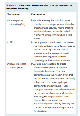
The second ML building block is feature engineering. The word ‘feature’ is typically interchangeable with ‘variable’ or ‘independent variable’. Model performance depends on the appropriate selection and inclusion of input features. An important consideration is the number of features in relation to the size of training subset where a larger number of features requires exponentially larger sample size (i.e. called ‘curse of dimensionality’). Thus, it is important to use appropriate feature selection techniques to remove irrelevant features that might simply introduce noise into predictions while ensuring that relatively important features are not omitted. Table 4 summarizes the commonly used feature selection techniques in ML. While most techniques for feature selection are data driven, it is worth noting that ML engineers should seek domain experts’ advice for identifying subsets of features that are mechanistically linked to predicting the outcome at hand,30,31 an approach that has been shown to significantly improve model performance.32
Table 4
Common feature selection techniques in machine learning
The third and most critical ML building block is model development. The starting point of this process is typically a partition of the dataset into a training subset and a testing subset. The ratio of this split is arbitrary and is frequently based on sample size. Common partitioning splits seen in clinical research include 70%/30%, 80%/20%, or 90%/10%. These two parts are disjoint with regard to a chosen variable (e.g. subject identifier, time of observations, etc.). The most important consideration is to make sure data from the same subject do not end up in both training and testing subsets (i.e. data leakage bias). When possible, the partitioning is done in a random fashion and at least preserves the prevalence of data samples per each class in the testing subset in comparison with the target population for which the model will be used. However, many data scientists elect to artificially keeping the prevalence of disease at ∼50% in the training dataset by oversampling the positive class (cases) or under-sampling the negative class (controls). This dataset balancing technique is meant to counteract false predictions caused by the algorithm’s over-reliance on the probabilistic distribution of the dominant class. For instance, in an unbalanced dataset with disease prevalence of only 10%, the algorithm would learn to predict ‘no disease’ whenever the uncertainty is high because there is a 90% chance this prediction would be true. Thus, balancing the training dataset can improve the classification performance during model development, although this can adversely affect generalizability to real-world data.
After the partitioning, the testing subset is set aside and not touched till ‘lockdown’ models have been obtained. To obtain lockdown models, training data are used. Using the whole training dataset for this task is impractical because a single training set is insufficient to find optimal hyperparameters or to assess variability in performance or risk of overfitting. Thus, to build more reliable lockdown models, the training subset is further partitioned into k-folds to use as cross-validation (CV) folds. These folds need to be created with proper stratification to maintain approximately equal ratios between positive and negative classes. The most used number of folds is 10 (i.e. 10-fold CV), which would allow adequate statistical comparison between variations in performance induced by different choices of parameters across these 10 folds. This is done in a round-robin way where the model is trained with nine folds (or k-1) and tested on the remaining fold. In each of the 10 iterative rounds, a different combination of hyperparameters is used (i.e. grid search). A performance metric [e.g. area under receiver operating characteristic (ROC) curve] is computed for each of the 10 folds and one-way ANOVA is used to determine whether different combinations of parameters have a statistically significant impact on performance. Next, the model (or models) that produces the highest average performance rank across the 10 CV folds is chosen and a final lockdown model is trained on the full training subset under the selected hyperparameters.
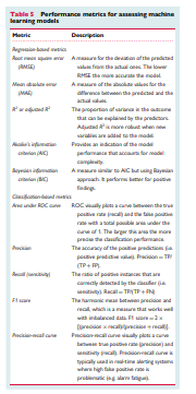
It is worth noting that if the training subset is not large enough to yield reliable distribution ratios in k-folds, the above procedure is modified by using an alternative CV approach referred to as leave one out cross-validation (i.e. LOOCV). In this approach, the grid search for selecting the hyperparameters for the lockdown is iteratively developed on n-1 training subsets and keeping that last subject in each iteration for parameter fine tuning. In either approach (k-fold CV or LOOCV), the final lockdown model is validated on the hold-out testing subset to assess how learned prediction rules generalize to new data and obtain final performance metrics. Table 5 summarizes the standardized performance assessment metrics used in predictive analytics.
Table 5
Performance metrics for assessing machine learning models
The above procedure for partitioning the dataset during model development is used to assess for overfitting; the biggest challenge in building a valid and generalizable ML model. Overfitting implies that the algorithm has captured patterns in the data irrelevant to outcome of interest (e.g. confounders, redundancy, missingness, outliers, etc.) rather than the real associations between variables. Such ‘noise’ causes the model to overfit the training data, so it generalizes poorly to new data (Figure 7A). To assess for overfitting, one first must estimate the overall bias in model predictions during training and compare it to the associated variance during testing. Bias refers to the overall model accuracy on historical data (e.g. root mean square error for regression, area under ROC curve for classification), whereas variance refers to the consistency in performance on future data. There is a tradeoff between bias and variance (Figure 7B). This means that very accurate models during training could yield large prediction error on new data (low bias — high variance), whereas less accurate ones during training could generalize well on new data without loss in performance (high bias − low variance). These challenges emphasize the need for evaluating a suite of regressors or classifiers during model development before selecting the model that best fits the data (i.e. optimizes bias − variance tradeoff).
Figure 7
7a — Such ‘noise’ causes the model to overfit the training data, so it generalizes poorly to new data
7b — There is a tradeoff between bias and variance
Overfitting and bias-variance tradeoff in machine learning model development. (A) The simple classification case of a binary outcome (denoted by diamonds and circles) using two variables X1 and X2. Unlike the first two classifiers that focused on capturing a real association between X1, X2, and the outcome, the last classifier seemed to capture patterns in the data irrelevant to outcome of interest (e.g. confounding, redundancy, missingness, outliers, etc.), thus ‘overfitting’ the model to training data. In (B), the plot to the left demonstrates three dynamic phases of the tradeoff between bias (training error) and variance (testing error): low bias − high variance (overfitting), low bias — low variance (optimal fitting), and high bias — high variance (underfitting). The two plots to the right show the area under receiver operating characteristic curve of three classifiers (C1, C2, and C3) fitted on a training cohort of n = 745 and testing cohort of n = 499.32 C1 shows the lowest bias (high area under receiver operating characteristic) during training but high variance (low area under receiver operating characteristic) during testing (i.e. overfitting), whereas C3 shows the highest bias (low area under receiver operating characteristic) during training and highest variance (low area under receiver operating characteristic) during testing (i.e. underfitting).
When training a deep neural network with stochastic gradient descent, the risk of overfitting is high. Therefore, at each round of training, it is typically necessary to further reserve a certain amount of data (10% of training data used in this round) as a validation dataset and to stop further gradient descent when a chosen performance metric or simply the value of the loss function stops improving after a set number of training epochs. Another challenge in training a deep neural network is the high cost in terms of computational power and therefore a random grid-based search of hyperparameters cannot be done with very fine resolution using an affordable amount of resources. Therefore, more recent approaches around AutoML need to be adopted where more effective ways of exploring the hyperparameter space can be achieved via algorithms such as genetic algorithm or Bayesian model optimization.
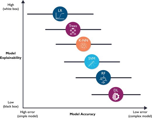
The fourth and final ML building block is prospective validation and integration into clinical workflow, which are not trivial tasks. Implementation into clinical workflow requires system training, performance engineering, monitoring, and system updating.33 More importantly, before any implementation, ML models require unique considerations for evaluation for optimal clinical utility, including prospective validation in representative clinical settings, as well as establishing benchmarks against reference standards. Unfortunately, almost 80% of DL-based models are based on open-source datasets.34 Nearly half of studies carried out in representative clinical settings show no incremental diagnostic gain over existing clinical decision support tools.35 These observations suggest a need for more sophisticated models to warrant a change in clinical practice. However, it is worth noting that the improved accuracy which accompanies increased model complexity also accompanies diminished model explainability. Figure 8 shows a hypothetical tradeoff between model accuracy and mode explainability. Explainability here refers to a human’s ability to understand the algorithm’s ‘logic’ (e.g. how and why a certain class was assigned). Explainable ML models are essential in healthcare not only because of their compatibility with clinical workflow and bedside care, but also for improving rigour and reproducibility of clinical investigation. There are currently numerous ‘under-the-hood’ techniques to improve ML model explainability, including partial dependence plots, rule extraction (e.g. fuzzy rules), feature importance (e.g. local interpretable model-agnostic explanations or LIME), decision trees, sensitivity analysis, layer-wise relevance propagation, and attention mechanisms (e.g. heatmaps).36–38
Figure 8 — shows a hypothetical tradeoff between model accuracy and mode explainability.
Hypothetical tradeoff between model accuracy and model explainability. This figure shows a hypothetical relationship between model accuracy (computational cost) and model explainability. It is worth noting that this is an over-simplistic view of the relationship between these two constructs, and that the relationship between the selected classifiers is not linear. Yet, this figure emphasizes that predictive modelling is ‘mission critical’; explainable (simple) models are preferred because they will be trusted more, and thus used more.11 These models might also be more accurate than complex ones (note the horizontal error bars for accuracy). DL, deep learning; RF, random forest; SVM, support vector machine; K-NN, nearest neighbours; LR, logistic regression.
Methodological considerations for design rigour
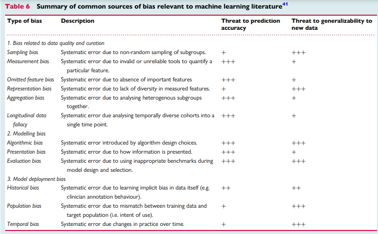
A main challenge in any scientific inquiry is ensuring that conclusions are valid and reliable. This implies that published results must be reproducible.8 Unfortunately, more than 70% of scientists failed in replicating others’ findings and nearly half failed in reproducing their very own findings,39 making bias, or systematic errors, an unprecedented threat to evidence-based practice.40 Using robust experimental workflows to reduce unintentional errors is at the heart of scientific inquiry principles. There are numerous types of bias specific to ML literature. Table 6 summarizes numerous sources of bias relevant to ML research as previously identified by Mehrabi et al.41 In this table, we also relate the magnitude of threat of each source of bias to prediction accuracy of the ML model and its generalizability to new data.
Table 6
Summary of common sources of bias relevant to machine learning literature41
Herein we highlight few sources of ML bias that are closely related to healthcare research. The first important methodological consideration is the impact of study design on ML models. Most ML models are developed on historical data from observational research (cohort and case–control designs). Each of these designs bring inherited methodological limitations on data quality and potential clinical use. While cohort studies are methodologically suitable for disease prognosis (forecasting) and diagnostics (predictive analytics), case–control studies are less reliable for designing predictive analytics. Specifically, predictive models developed on case–control studies were poorly calibrated and had less discriminative power when compared with cohort studies for modelling the same outcome.42 This poor performance can be attributed to poor control over known and unknown confounders during the selection of samples in case–control designs, emphasizing that careful construction of a case–control design can lead to comparable discriminative performance as a cohort design. Other limitations for the poor model calibration in case–control designs are (i) the over-representation of the outcome class, (ii) the poor representation of data available during the time of diagnosis, and (iii) the overemphasis on features closer to the outcome of interest (temporal bias).43 Thus, a ML model based on case–control studies must be prospectively validated using a cohort design for fair evaluation and recalibration before any clinical deployment.42
A second important consideration for ML applications in healthcare is sampling bias. Although most ML engineers focus on the adequacy of training samples and the numeric distribution of input features, little attention is paid to the sampling techniques used to collect the historical data in the first place. If biased sampling techniques were used, then the probabilistic distribution of features in training data might be different than that in representative clinical settings.44 This might produce models that are not only poorly generalizable to unseen data, but also lack physiological plausibility. Another important sampling concern is using multiple samples from the same patient across training and testing subsets. Unless these multiple samples are physiologically distinct, then the modelling dataset would be flawed. An example would be using each heartbeat within a 10-s ECG rhythm strip as a training sample. This essentially violates the Gaussian distribution principles where input features are expected to be independent and identically distributed. This frequently yields unrealistic and exaggerated performance metrics during model training, which would again poorly generalize to new unseen data.
Another critical consideration in ML research is the rigour of the ascertainment of the outcome variable. The conclusion validity of any supervised ML model depends heavily on the quality of labels on which the model was trained. High-quality labels need to be based on a good reference standard (e.g. gold standard) or a majority panel vote (e.g. consensus adjudication) where reviewers are blinded to model predictions.45 Poorly labelled outcome data will negatively affect model building twice, once during model training and once during model evaluation, leading to high bias − high variance tradeoff. Moreover, given that sophisticated ML models require large amount of data, many studies rely on ‘silver’ labels. Outcome ascertainment using silver labels can be based on with electronic health records (EHR)-phenotyping (i.e. rule-based queries) or semi-supervised labelling (i.e. predictions by active learning), each of which comes with its own limitations. For example, EHR-based phenotyping has been shown to miss up to 21% of acute MI events.46 Thus, assessing the quality and robustness of outcome ascertainment is important before evaluating model performance claims.
Quality assessment checklist
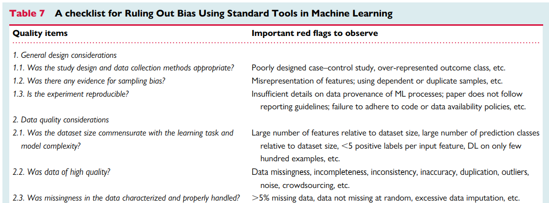
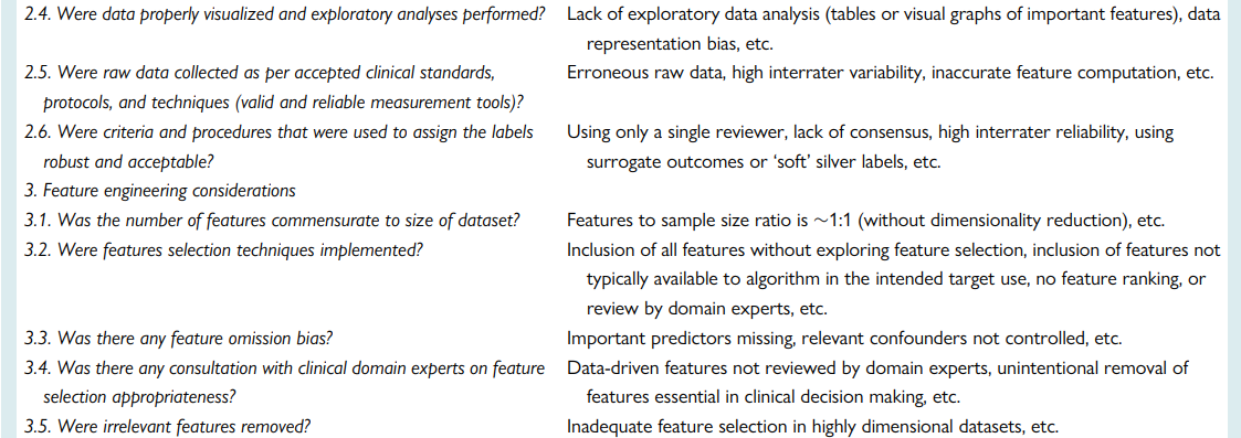
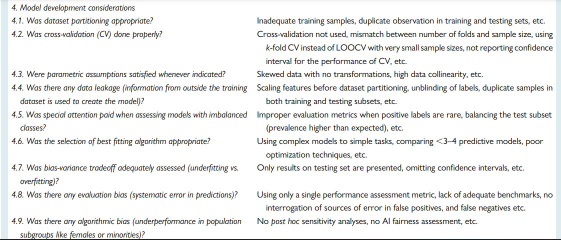
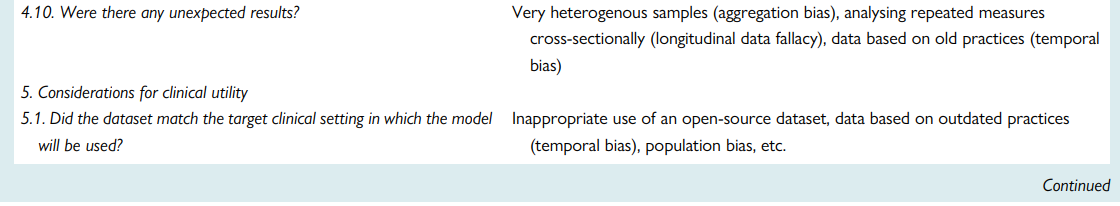
Ensuring rigours and reproducibility in ML research is essential for designing functional algorithms for clinical use, and there are currently numerous reporting guidelines and user guides for designing such ML models.1,8,33,45,47–52 However, evaluating the quality of a published ML paper requires a comprehensive understanding of the available ML techniques and approaches; the main building blocks of a functional ML pipeline; and potential design flaws and methodological biases involved. Table 7 provides a summary checklist for systematically evaluating published ML studies. This checklist can guide clinicians while evaluating the rigour of a published ML study by asking the most relevant questions and searching for potential pitfalls and red flags.
Table 7 — A checklist for Ruling Out Bias Using Standard Tools in Machine Learning
Summary
Developing functional ML-based models to address unmet clinical needs requires unique considerations to reach the stage of potential clinical utility.
This review summarized the main ML building blocks and identified important red flags clinicians should observe while critically appraising ML applications in healthcare.
Bridging the gap between clinicians, healthcare scientists, and ML engineers can address many shortcomings and pitfalls of ML-based solutions and their potential deployment at the bedside.
It is important for clinical ML studies to be reviewed by clinicians, and a checklist such as the one provided herein may serve as an aid.
It is worth noting, though, that this checklist requires subsequent revisions using a formal Delphi consensus process so that it can be listed on the EQUATOR Network as a formal quality assessment tool.
References and additional information:
See the original publication
About the authors & affiliations
Salah S. Al-Zaiti 1 * Alaa A. Alghwiri 2 , Xiao Hu 3 , Gilles Clermont 4 , Aaron Peace 5 , Peter Macfarlane 6 , and Raymond Bond 7
1 Department of Acute and Tertiary Care, Department of Emergency Medicine, and Division of Cardiology,
University of Pittsburgh, Pittsburgh PA, USA;
2 Data Science Core, The Provost Office,
University of Pittsburgh, Pittsburgh PA, USA;
3 Center for Data Science,
Emory University, Atlanta, GA, USA;
4 Departments of Critical Care Medicine, Mathematics, Clinical and Translational Science, and Industrial Engineering,
University of Pittsburgh, Pittsburgh, PA, USA;
5 The Clinical Translational Research and Innovation Centre, Northern Ireland, UK;
6 Institute of Health and Wellbeing, Electrocardiology Section, University of Glasgow, Glasgow, UK; and 7 School of Computing,
Ulster University, Ulster, UK
Originally published at https://academic.oup.com